How to value options

We can not value option in the way we do for other financial assets so by calculating the expected cashflow and discounting it using the opportunity cost of capital. We can calculate the expected cashflow of an option but it is impossible to calculate the opportunity cost of capital because it changes every time the stock price moves. Because when you buy a call option you are “using” the stock without really owning it, the option is much riskier than the stock on which is based meaning that it has higher beta and its returns have higher standard deviation. The option is more risky when the actual price of the share is lower than the exercise price with respect to an option based on a stock that is actually traded at a price higher than the exercise price. If the price of the stock increases, its expected payoff if higher while its risk is lower.

SO HOW DO WE VALUE OPTIONS?

In order to value options we could create a combination of stocks while borrowing money that has the same cost as the option. This is because, because of the law of one price, investments having the same price have the same expected return. Imagine that we are again considering a stock trading at $500 which is expected in six months to increase its value up until $600 or to decrease it until $450. Suppose also that the risk free rate is 2% for six months. If the price falls, the option is obviously worth nothing but, if the price rises, the option will be worth: $600-500=$100. Now, if we bought 2/3 of the share and borrowed the NPV of $300 from the bank we would obtain: 0 if the option would result worthless (because we would just have to payback the debt with no profits) or 2/3*600-300=100 in case the price rises. So we have successfully emulated the performance of the option using assets that we know how to value. Since the payoffs of the option and of our financial instruments is the same we can say that:

Value of the call = Δ*shares – value of the bank loan = 2/3*500-300/1.02= 39.22

The technique we just used is called replicating portfolio and the number of shares necessary to replicate it is called option delta.

To calculate how much debt you need to use, you have to set:

And just solve to find debt. In our case we would have:

100 = 2/3*600 – debt

debt = 2/3*600 – 100 = 150

Another method

Our call should have been priced at exactly its value: $39.22. To understand why, suppose that the price was higher than that. If this was the case, you could earn a profit by buying 2/3 of the share, borrowing the present value of $150 and selling the option. Conversely, suppose that the price was lower than $39.22. In this case, you could make a profit by lending the money instead of borrowing it, selling the 2/3 of the share and buying the call option. This would mean having an arbitrage opportunity that is impossible in an efficient market. The option price does not depend on the attitudes investors in the market have toward risk. Because of that, we can calculate the value of an option thinking that all the investors are indifferent about risk. If this is the case, each cashflow and each financial instrument will have the same cost of capital and discount factor equal to the risk free rate of return. In our example, it would mean that the expected return that investors expect on the stock is equal to 2% for six months. We assumed that our stock can either increase its price by 20% or it can reduce it by 10%. By using this data we can calculate the expected probability that the stock will rise (p) and the probability that it will fall (1-p) by setting:

By solving the computations we find p=0.4 and 1-p=0.6. Remember that this probability is computed using the imaginary world assumption that the expected return demanded is the same as the one demanded for risk free assets. In reality, the return demanded is obviously higher and so is the probability p. In general, the formula for calculating p can be written as follows:

Which in our case is:

By using these probabilities we can find the expected value of the call as:

Which in our case is:

0.4*100 + 0.6*0 = 40

Now we discount it using the cost of capital:

So we obtained the same result as before!

SAME METHOD, DIFFERENT OPTION

Let’s use the same assumptions as before: the actual price of our stock is $500 and it can either increase to $600 or decrease to $450. This time however, if the price increases, the option will have no value while if the option decreases in value it will have a value of: $500-450=$50. Let’s calculate the option delta:

The option delta is always negative when considering put options. This is because you need to sell stocks while lending money this time to mimic the option. Once again to find the amount you have to lend you just set:

And just solve to find receivable. In our case we would have:

50 = -1/3*450 + debt

debt = 50 + 1/3*450 = 200

To successfully imitate the option you should sell 1/3 of the share and lend the present value of 200. This is because, in case the stock price increases you will sell the shares at a price of 1/3*600=200 (thus your portfolio will be worth $200 less) but you would receive the $200 from the loan so the total change is 0. If instead, the price of the stock decreases to 450, you will sell your 1/3 of it for $150 but you will receive the $200 from the loan, so the total change is +$50. Because the investments have the same payoffs they must have the same value:

Value of the put = Δ*shares + value of bank loan= (-1/3) *500+200/1.02=29.41

Now, let’s try to value the option using the risk neutral method. We can use the probabilities calculated with the call option since the assumptions are the same. So p=0.4 and (1-p)=0.6. The expected value of the put option will be:

0.4*0 + 0.6*50 = 30

Now to find the current value of the put option just discount for the risk free rate:

We can also check now that the fundamental relationship for European option holds:

Value of put = value of call + present value of exercise price – share price

Value of put = 39.22 + 500/1.02 – 500 = 29.41

THE BINOMIAL METHOD

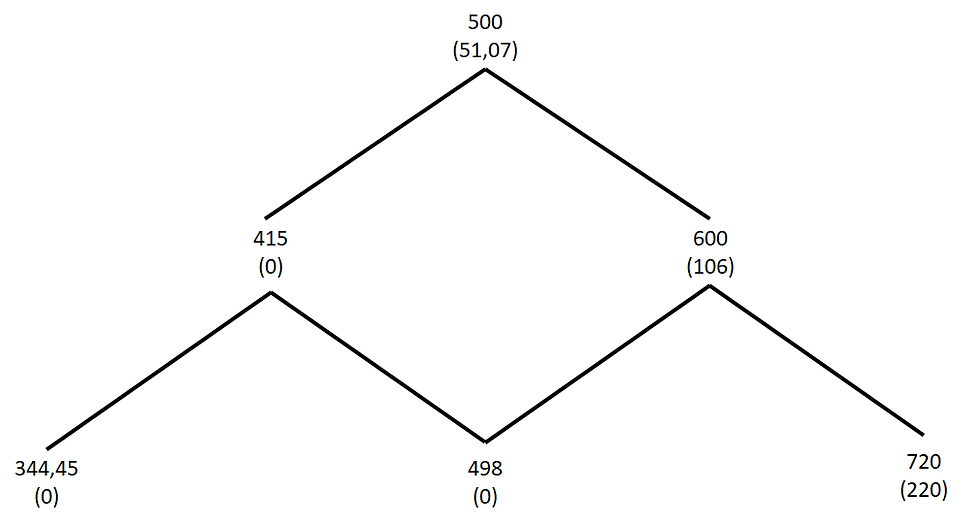
The last example used a simplified version of the so called binomial method. This method is based on the assumption that the stock price can move in only two directions: up and down. Now, we assumed in last examples that the stock price changed only one time during the 6 months but now, to make things a little bit more realistic, we could decide to take shorter intervals in which this price can change. We could for example assume that the price of the stock changed once every 3 months. By doing so, we are giving to the possible values the stock reaches after 6 months more variety. We could continue to divide out 6 month period in infinite parts until we arrive to a situation in which the stock price changes constantly like in reality.

Now, we could use both the replicating portfolio method or the risk neutral one. However, if we use the replicating portfolio method we should calculate a different option delta for each node of the tree. It is convenient to do so only if we have a small number of nodes. If we have a lot of nodes it more convenient to use the risk neutral method. Let’s assume that every 3 months the price of the stock can increase by 20% if or decrease by 17%. We assumed an interest rate of 2% so, for a three months period, the interest rate will be approximately 1%. The probability that the stock rises is given by:

So we have a chance of 48.649% that the stock will increase its value and a chance of 51.351% that the stock value will decrease. We can also check that it is the case:

0.48649*(20)-0.51351(17) = 1

Which is exactly our risk free interest rate. Suppose we are in the third month and that our stock in the first 3 months increased its price to $600. We know that our stock in the following 3 months can be worth $720 or $498 so the option will be worth $220 or 0. We can once again use the probabilities that the stock will rise or fall to find the expected value of the option at the end of the period.

0.48649*(220)+0.51351(0) = 107.03

Because we are in the third month but we are considering cashflows from the sixth month, we need to discount the expected value: 106/1.01=106

If instead our stock decreased in price in the first 3 months, now it can either increase its value to $498 or its value can fall again to $344.45. Our option will therefore always be worth 0.

Therefore we know the possible values of the option in three months from the present: $106 or 0. Now we can calculate the value that the option has in the present using those values:

0.48649 *106+0.51351*0=51.568

Once again we are considering values three months from the present and, because of that, we have to discount them: 51.568/1.01=51.057.

Here are the various steps graphically:

INSIGHTS

The binomial method is a better way to calculate the value of an option because stock prices change constantly and, by using intervals of time small enough we can become more and more precise about the possible stock movements. You may ask yourself how we decided that the stock price would rise by 20% or decrease by 10%. Well there is a relationship that links the change of the stock price to its standard deviation and the number of small periods we are considering:

e is the Euler’s number and is equal to 2.718

σ is the standard deviation of the stock

h=interval expressed as a fraction of one year.

In our computations we assumed that the standard deviation of the company’s stock was: 0.36.

So: