CAPM

Generally, if you measure the returns on stocks over a short period of time conform in a way close to a normal distribution. A normal distribution is peculiar relationship among two variables. In our case, the two variables are the expected value of the stock and its standard deviation or variance. In the figure are shown 3 different investments: A and B have the same expected value but B has a lower standard deviation because most of the times the data were close to the expected value. C has the same standard deviation as B but a higher expected value.

PORTFOLIOS MADE UP OF STOCKS

If you have two stocks A and B and you want to build your portfolio, you can choose various combinations of them. How you compose your portfolio will determine its expected return and its standard deviation. Imagine that A has an expected return of 5 and a standard deviation of 7 and B has an expected return of 15 and a standard deviation of 13. If your portfolio is made up half of firm A’s shares and half of firm B’s shares. The expected return of the portfolio and its standard deviation will simply be computed as the weighted average of the stocks composing it. So in our case it will have expected return of 0.5*5+0.5*15=10 and a standard deviation of 0.5*7+0.5*13=10. Remember that in general you are differentiating to reduce risk but you reduce risk only in the case in which the stocks are not perfectly correlated (ρ=+1). In the picture is represented a relationship among various combinations of two stocks with their corresponding standard deviation and expected return. The red dotted lines represent the unrealistic case in which the stocks are perfectly negatively correlated (ρ= -1). If this happens, your portfolio carries no risk at all.

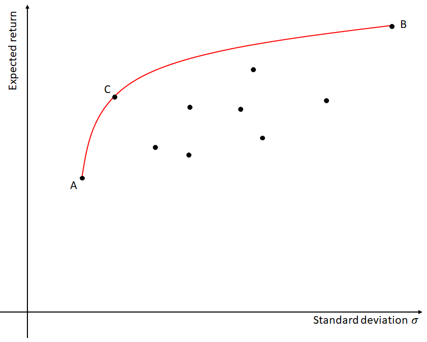
We considered a simplistic example, in reality you can create your portfolio with more than two stocks. Consider an example in which you are investing in a portfolio of 10 stocks like in the picture like in the picture below. In this case you expand your possibilities and you can obtain more risk-return combinations than before. The red line in the picture represents the so called efficient portfolios. An efficient portfolio is a portfolio that offers the highest possible return given the level of risk you are willing to bear. In order to find the set of efficient portfolios, you need to use a quadratic computer, the standard deviation and the expected return of each stock.

BORROWING AND LENDING

Investors can generally borrow but also lend money at a risk free interest rate that we are going to denote with rf. If you decide to invest in an efficient portfolio like portfolio M by borrowing or lending your money at that risk free rate, you will be able to obtain any combination of risk and return represented by the line in the picture connecting the rf and your portfolio. When you lend your money instead of investing them in the portfolio the combination of return and standard deviation you can obtain is in between rf and M while if you borrow money using that risk free rate you will be able to increase your possibilities of return beyond M.

Notice that some portfolios represented in the picture don’t make sense: why would you for example invest in the portfolios in the blue part of the line if there are other portfolio that offer higher expected returns while bearing the same risk? In out example M is not only an efficient portfolio, it is the best efficient portfolio. It is the best efficient portfolio because it offers the highest ratio of return over risk. This ratio computed as the risk premium over the standard deviation is called the Sharp ratio:

When you have the graph of the efficient portfolios you can find the best efficient portfolio as the tangency point between the line starting from rf and the curve of those efficient portfolios.

HOW RISK AND RETURN ARE RELATED

We are using treasury bills as our example of safe investments. As such, they have a β=0 because they are unaffected by any of the market movements. When you are willing to invest in riskier assets you will also earn the possibility to get higher expected returns. The difference between the expected return that you can get by investing in the market and the return you can get by investing in risk free assets is called the market risk premium (rm-rf).

On average in past years the risk premium is estimated to be 7.7% a year. In a competitive market, the risk premium varies with the beta of the stocks you buy. The higher the beta of a stock the riskier it is and the higher are its expected returns. The risk return therefore depends on the beta. We can represent this relationship using a line called the security market line. This method of estimating the return and therefore the value of an asset depending on his beta is called the capital asset pricing model (CAPM). According to the linear relationship depicted by this model, the return of a stock having beta 0.5 is exactly half the one of the market and the return of a stock having beta 2 is exactly double the one of the market. The expected risk premium can therefore be computed as the beta rimes the expected risk on the market:

In a well functioning market, there will be enough investing possibilities for investors so that the expected returns on assets which are equally risky are all the same. The CAPM predicts that the risk premiums of stocks should increase following the linear relationship depicted but, by looking at history we can see that riskier stocks on average had higher returns than non risky ones but not as good as the CAPM predicts. You could therefore think that the CAPM is not very accurate but, in reality, you have to remember that the CAPM deals with expected returns, not actual returns. The actual returns of stocks can be influenced by a lot of factors like expectations, opinions, socio-political situations and that therefore are subjected to some “noise”.