Cost curves for a firm

In this lecture we are going to explore how a firm can represent and analyse its own costs. In order to fully understand that lecture it is suggested to read the previous one on cost and cost minimization.

COST CURVES IN THE LONG RUN

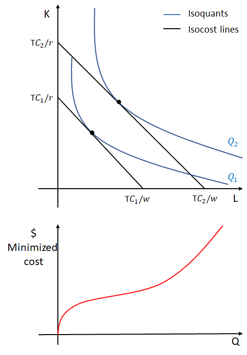
When a cost minimizing firm decides to produce more output we shift the isocost line farther from the origin, because, the more the firm wants to produce the higher will be the total cost it will have to pay and the farther the isocost line will be from the origin. In order to represent how the firm’s minimized total cost will change in the long run depending on the output the firm wants to produce, we use the long run total cost curve denoted by TC(Q) meaning that the firm’s total cost is a function of Q. Obviously the curve will be sloping upward indicating a positive relation between TC and Q (meaning that if Q increases also TC will increase) and will start from the origin because, in the long run, the firm has no fixed sunk costs and therefore if the firm produces 0 output the total cost will also be 0.

WHAT HAPPENS WHEN THE PRICES OF INPUTS CHANGE?

We have discussed yet in the lecture about the cost minimization problem that an increase in the price of at least one input always increases the firm’s total cost. If only one input changes in price or if both change but by different percentages the total cost for the firm will rise and the long run total cost curve will change in shape because the cost minimizing bundle of inputs will change. If, however, both inputs change in price by the same percentage, the cost minimizing bundle of inputs will not change (also this has been discussed in the lecture about the cost minimization problem). In this case the total cost curve will shift upward (not in a parallel fashion) by the same percentage by which both the inputs prices have increased. The curve will not shift in a parallel fashion because remember that, in the long run, if the firm produces no output, the total cost will be 0. An increase in the price of both inputs by 20% will shift the long run total cost curve upward by exactly 20%.

LONG RUN AVERAGE AND MARGINAL COST

We define the average cost per unit of output in the long run as the firm’s long run average cost. It is computed indicated by AC(Q) meaning that it depends on the quantity of output the firm wants to produce. It is computed as:

AC(Q) = TC(Q)/Q

The long run marginal cost represents instead by how much increases the long run total cost when increasing the quantity of output by 1 unit. It is indicated by MC(Q) and it is computed as:

MC(Q) = (ΔTC)/(ΔQ) =𝜕TC/𝜕Q (the derivative of TC with respect to Q)

Graphically you can think of AC(Q) as the slope of a ray starting to the origin and crossing the TC(Q) function at value x-value Q while MC(Q) can be interpreted as the slope of TC(Q) itself. Notice that, when the average cost is higher than the marginal cost, average cost is decreasing and, when the average cost is lower than the marginal cost, average cost is increasing. Marginal cost and average cost intersect exactly at the minimum of the average cost.

ECONOMIES OF SCALE

When a firm can reduce average cost by increasing the output produced, the firm is said to enjoy economies of scale. The opposite situation called diseconomies of scale is experienced by the firm when, as the output produced goes up, average cost goes up as well. At first, the long run average cost curve is decreasing as output increases meaning that the firm is enjoying economies of scale. This happens because often firms have some fixed costs that are output insensitive meaning that they do not change if a firm produces more or less output. By producing more output the firm is able to “distribute” that cost over more inputs. Imagine that your factory needs to be heated up to a certain temperature and that in order to do that you have to spend 100$ a day. If you produce during the day 10 units of output the cost of heating up the factory per unit is 100/10=10$. If during the day you produced

20 units of output, the cost of heating up the factory per unit is 100/20=5$. The minimum quantity at which the average cost is minimum is called minimum efficient scale (MES). After that point the average cost stays the same even if the quantity produced increases. This area is the one of constant returns to scale. The average cost then starts increasing again and, as said, the firm suffers from diseconomies of scale. This happens because firms often can not manage effectively its production causing therefore managerial diseconomies that lead to an increase in costs.

COST CURVES IN THE SHORT RUN

Just like the long run total cost curve the short run total cost curve STC(Q) depicts the relationship between the quantity the firm wants to produce and the total cost it has to bare. Because we are in the short run, the firm has some fixed costs that can not be avoided (sunk). Let’s suppose once again that the firm’s quantity of capital used is fixed at Ḱ. The firm’s short run total cost is the sum of two components:

• Total variable cost TVC(Q) which depends on the quantity produced.

• Total fixed cost TFC which but it is fixed at rḰ (the quantity of fixed capital times its price). It does not depend on the quantity produced and, because of that, graphically it represented as an horizontal line.

Because the firm has some fixed costs the curve will not start from the origin but from the point (0, r Ḱ). The short run total cost curve is higher than the long run total cost curve because the firm can not freely control the quantity of inputs employed. The only case in which the two curves touch is where the quantity at which the capital employed is fixed is exactly the one the firm would have chosen if it had no constraints. Only in that case the long run and short run total costs are equal.

SHORT RUN AVERAGE AND MARGINAL COST CURVE

Just as in the long run, the short run average cost is a curve representing how the average cost per unit in the short run changes as the quantity produced changes. It is defined as:

SAC(Q) = STC(Q)/Q

Also the short run average total cost is the sum of two components:

• Average fixed cost computed as: AFC = TFC/Q and it is always decreasing as Q increases.

• Average variable cost computed as: AVC = TVC/Q which decreases at first and then increases again becoming closer and closer to the average total cost (because, as said AFC, becomes closer and closer to 0).

The short run marginal cost represents instead by how much increases the short run total cost when increasing the quantity of output by 1 unit. It is indicated by MC(Q) and it is computed as:

MC(Q) = (ΔTC)/(ΔQ) =𝜕TC/𝜕Q (the derivative of TC with respect to Q)

And, just like in the long run, the short run marginal cost can be graphically thought as being the slope of the short run total cost curve.

RELATIONSHIP BETWEEN LONG RUN AND SHORT RUN AVERAGE AND MARGINAL COST CURVES

As we have seen, both the short run and long run average curves are U-shaped. The short run average cost curves are higher than the long run one because of fixed costs and that they touch only when particular conditions happen. If you consider a high number of short run average cost curves you would notice that they would approximate the shape of the long run average cost curve. This means that you can consider the long run average cost curve as the envelope containing an infinite number of short run average cost curves.