Production with two inputs

A PRODUCTION FUNCITION CONSIDERING MORE THAN ONE INPUT

Consider a firm using as inputs labor (L) and capital (K). In order to represent graphically the quantities of labor and capital employed and the output (Q) produced we need a three-dimensional graph called the total production hill. On the x and y axes are represented the quantities of the inputs while on the z axis it is indicated the quantity produced by the firm (the higher is the total production function the higher the quantity produced).

Notice that, if you fix the quantity of capital at a specific value and consider how the quantity produced changes when changing only labor, you are going back to a total product function; therefore a total production function (with respect to labor) can be derived from a total product hill by fixing capital at a particular level. Notice also that the total product hill respects the law of diminishing marginal returns: if you fix capital at a specific level and consider once again how Q changes with L, you will move along the total production hill in a parallel fashion with respect to the x axis (look for example at the green line in the graph). As you can see the quantity produced at first increases rapidly, then it continues to grow always at a slower pace until it starts decreasing. When you consider a two-inputs production function, in order to compute the marginal product of one of the inputs you have to keep the other one as constant. The marginal product of labor is computed as:

The marginal product of capital is computed as:

ISOQUANTS

An isoquant is a curve that represents how you can substitute L and K while keeping the quantity of output as constant. Along an isoquant the quantity produced by the firm is the same. You can think of cutting the total production hill at a specific z-value (Q) and projecting it on a two dimensional graph. This means that isoquants which are nearer the origin represent lower quantities produced. The number of isoquants is infinite and each one of them corresponds to a specific level of output. The farther is the isoquant from the origin, the higher is quantity produced by the firm along that isoquant. We have to distinguish between economic and uneconomic regions when representing an isoquant. In the economic region of production, the isoquant is downward sloping meaning that if you use more labor you can use less capital and vice versa. Remember that not always increasing an input will means an increase in quantity produced too (did you miss the lecture on production with only 1 input?). When the quantity used of an input is too much it could happen that the total quantity of output will decrease. This is represented graphically by the uneconomic region of the graph. Notice that, when K becomes too much and we have diminishing marginal returns to capital (MPk < 0), in order to remain on the same isoquant, we have also to increase labor to compensate for the negative effects of too much capital and therefore the isoquant bends to the right and becomes upward sloping. The same reasoning can be done considering labor. When L becomes too much and we have diminishing marginal returns to labor (MPL < 0), in order to remain on the same isoquant, we have also to increase capital to compensate for the negative effects of too much labor and therefore the isoquant bends upwards and becomes once again upward sloping.

HOW YOU CAN SUBSTITUTE THE TWO INPUTS WHILE KEEPING OUTPUT CONSTANT?

In order to determine how much capital you have to employ when reducing labor while keeping output constant, you have to determine the marginal rate of technical substitution of labor for capital. It is denoted by MRTSL,K and graphically it measures how steep the isoquant is.

The property of diminishing marginal rate of technical substitution says that: if you consider a standard-shaped isoquant you can see that, as you move along the curve (from the left to the right), the slope of the isoquant becomes less negative (the curve becomes flatter). If curves present this property, they are convex to the origin. The marginal rate of technical substitution is defined as:

To understand why consider that, because we are on an isoquant, the quantity produced does not have to change as we move along it. This means that the quantity you “lose” because you employ less machinery has to be compensated equally by the quantity you produce by employing more labor. So in the end the change in the quantity produced must be 0. The quantity that you “lose” because you employ less capital is defined as: ). This is because MPK represents the quantity produced thanks to 1 unit of capital and represents the amount of capital we are deciding not to employ anymore. The quantity that you produce more because you employ more labor is defined as: ). This is because MPL represents the quantity produced thanks to 1 unit of labor and represents the amount of capital we are deciding to employ more. Because the total change in quantity has to be zero:

If we divide everything by MPK and ΔL we can rearrange the equation to:

But remember that the slope of a curve is defined as the change of the value on the y-axis over the change of the value of the x-axis. And therefore in out case: - ΔK/ ΔL =MRTSL,K. We can say therefore that:

THE SHAPE OF AN ISOQUANT

The shape of an isoquants depends on the substitution opportunities a firm has among its inputs. We can distinguish three cases:

• If a firm has little to no substitution opportunities the isoquants are L shaped and described thanks to a fixed proportion function. A general fixed proportion function has the form: Q = min (αL ; βK) where α and β are positive constants. The inputs involved in this kind of function are perfect complements. In this case the MRTSL,K is 0 on the vertical part of the isoquant, indefinite on the corner and 0 on the horizontal part and. The elasticity of substitution (the percentage change in K/L over the percentage change in the MRTSL,K) is 0. A firm which uses machines which are used by one or more people present this kind of function: a machine without a person controlling it is useless just like a worker without the appropriate tool.

• If a firm can substitute between the two inputs up to a certain degree the shape of the isoquant will be convex to the origin and often described thanks to a Cobb-Douglass function. A general Cobb Douglas production function has the form: Q = (AL^α )*(K^β) where α and β are positive constants and A is any number. The MRTSL,K varies along the isoquant and the elasticity of substitution is 1. Consider a farm t hat can use both people and machines to produce its vegetables. Even thought the firm can substitute one input for the other, it cannot be done until one of the two totally replaces the other because some men are required in order to control the machines.

• If a firm can perfectly substitute between the two inputs then the isoquants are straight lines and therefore described with a linear function. A general linear function has the form: Q = αL + βK where α and β are positive constants. The inputs involved in this kind of function are perfect substitutes. In a linear isoquant the MRTSL,K is constant and the elasticity of substitution is ∞ . Consider a company like Amazon. In order to organize the warehouse, it can employ men or robots. The substitution among these two inputs is fixed (for example a robot can replace 3 people) and one input can totally substitute the other.

RETURNS TO SCALE

If a firm uses two inputs: L and K and, if we increase simultaneously by the same proportion the quantities of both inputs used, then the quantity of output will increase. This links us to the concept of returns to scale. Returns to scale are defined as:

Suppose that you are increasing the quantity employed of both inputs by the same proportion ʎ (ʎ must be greater than 1 because otherwise you will reduce the quantities employed). Let Φ represent the percentage change in the quantity produced when increasing by ʎ the quantity of both inputs. We can distinguish 3 cases:

• If Φ > ʎ it means that the quantity produced increased proportionately more than the quantity used of both inputs. In this case we have increasing returns to scale. As you can see in the example in the picture, if we double the quantity used of both inputs, the quantity produced becomes more than twice the original one.

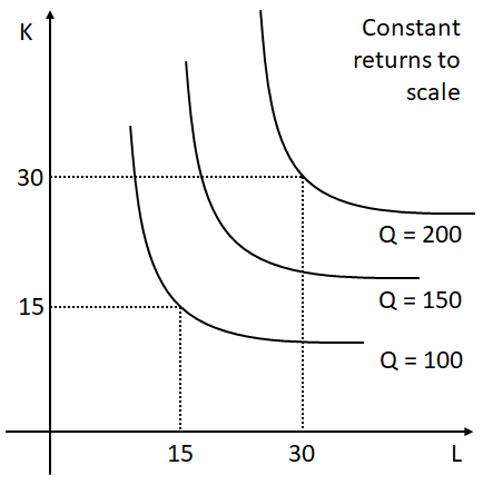
• If Φ = ʎ it means that the quantity produced increased by the exact proportion by which the inputs have increased. In this case we have constant returns to scale. As you can see in the example in the picture, if we double the quantity of both inputs, the quantity produced becomes exactly double the original one.

• If Φ < ʎ it means that the quantity produced increased proportionately less than the quantity used of both inputs. In this case we have decreasing returns to scale. As you can see in the example in the picture, if we double the quantity used of inputs, the quantity produced becomes less than twice the original one.

When a firm enoys increasing returns to scale, it has advantages from large-scale operations. This means that by keeping costs constant, a large firm will be able to produce more than a number of small firms that compounded are as big as the first one.

WHAT HAPPENS WITH TECHNOLOGICAL PROGRESS?

Production functions, and therefore isoquants can change over time. Technological progress is a situation in which a firm can produce the same quantity of output using a lower quantity of inputs (and therefore costs) or produce more by keeping costs constant. Once again we can distinguish three cases:

• Natural technological progress: in this case an isoquant corresponding to a given output shifts inward to the origin but the MRTSL,K along all the curve stays unchanged.

• Labor-saving technological progress: in this case the isoquant corresponding to a given output shif ts inward, this time the MRTSL,K changes: the curve becomes flatter, indicating that the MRTSL,K has increased (has become less negative). Remember that we defined MRTSL,K = -MPL/MPK, so if MRTSL,K increases the marginal product of capital increases more than the marginal product of labor.

Capital-saving technological progress: in this case an isoquant shifts inward, MRTSL,K changes : the curve becomes steeper indicating that the MRTSL,K has decreased (has become more negative).